Tutorial: Stable Diffusion from Scratch II
This is a regurgitation of the previous Tutorial: Stable Diffusion from Scratch. It's taking me much more than 1 day to understand and implement the code in that article. Accidentally, the original articles have been removed from the web - so as much as it is questionable that I have copy-pasted someone else's work - well, the original is no longer available, so mine may become an authoritative copy. And to be clear: I have deep admiration for the authors I copy. I am jealous of their mental agility and strength (and the time and resources they have available to pursue these research topics). I admire the people who invented stable diffusion, and other algorithms in its vicinity. Below is my humble attempt to reimplement the code from that paper, and get a stable diffusion instance, written from scratch, up and running.
Also, I will be mostly focusing on things I'm struggling with, so this may not be a full and complete tutorial. Additionally, for the reader, I strongly recommend this book: Dive into Deep Learning. Very clearly written; it's helped me a lot. Their explanation of the furier time encoding made the concept crystal clear for me. Now then, a quick table of contents for this article:
Table of Contents
- basic 1D forward/reverse diffusion
- a U-Net architecture for working with images
- the loss associated with learning the score function
- an attention model for conditional generation
- an autoencoder
Basic forward and reverse diffusion
For the architecture of stable diffusion. Let's say we have our data (images, or a single datapoint) and we add noise to it. We then train a neural network to denoise our data. So we will have forward diffusion (adding noise) and reverse diffisuion (removing noise). For a first step, we a very simple one-dimensional datapoint (y) that gets diffised as a function of time (x).
$$ x(t + \Delta t) = x(t) + \sigma(t) \sqrt{ \Delta t} \; r $$
Where \( \sigma(t) > 0 \) is the noise strength, \( \Delta t \) is the step size, and \( r \sim \mathcal{N} (0, 1) \) is a standard normal random variable. We repeatedly add normally-distributed noise to our sample. Often, the noise strength \( \sigma(t) > 0 \) is chosen to depend on time, and gets higher as t gets larger. This is a forward pass, so \( \sigma(t) \) gets larger with time when adding noise, and gets smaller with time when removing it.
Let's implement the forward pass in python.
## Simulate forward diffusion for N steps.
def forward_diffusion_1d(x0, noise_strength_fn, t0, nsteps, dt):
  """x0: initial sample value, scalar
  noise_strength_fn: function of time, outputs scalar noise strength
  t0: initial time
  nsteps: number of diffusion steps
  dt: time step size
  """

  # Initialize trajectory
  x = np.zeros(nsteps + 1); x[0] = x0
  t = t0 + np.arange(nsteps + 1)*dt

  # Perform many Euler-Maruyama time steps
  for i in range(nsteps):
    noise_strength = noise_strength_fn(t[i])
    random_normal = np.random.randn()
    x[i+1] = x[i] + random_normal
  return x, t

## Example noise strength function: always equal to 1
def noise_strength_constant(t):
  return 1
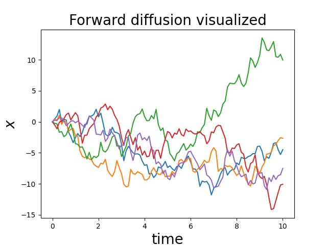
Let's run it and visualize it:
nsteps = 100
t0 = 0
dt = 0.1
noise_strength_fn = noise_strength_constant
x0 = 0

num_tries = 5
for i in range(num_tries):
  x, t = forward_diffusion_1d(x0, noise_strength_fn, t0, nsteps, dt)

  plt.plot(t, x)
  plt.xlabel('time', fontsize=20)
  plt.ylabel('$x$', fontsize=20)
plt.title('Forward diffusion visualized', fontsize=20)
plt.show()
We can reverse this diffusion process by a similar-looking update rule:
$$ x(t + \Delta t) = x(t) + \sigma(T - t)^2 \frac{d}{dx}\left[ \log p(x, T-t) \right] \Delta t + \sigma(T-t) \sqrt{\Delta t} \ r $$
Where
$$ s(x, t) := \frac{d}{dx} \log p(x, t) $$
- x = the noisy image at time t
- \( p(x, t) \) = probability density of x at time t
- \( \frac{d}{dx} \) = gradient with respect to x
- \( s(x, t) \) = the score function
This is a key conceptual point in diffusion models and Stable Diffusion. The goal of the model is to learn how to denoise x by moving it toward higher-probability regions of the data distribution. Why log(p) instead of p? This has numerical advantages. Probabilities p(x) are often very small, especially in high dimensions.
The derivative of a log of a small value is pretty large. Also, taking the log turns products into sums, making gradients more stable. The log gradient gives a direction rather than a magnitude that depends on the absolute value of p(x). log p(x) and p(x) are equivalent in optimization, but the former is much more stable numerically. Many learning algorithms (MLE, score matching) naturally use log.
And what does it mean to have a probability distribution of an image? For that, I refer you to variational auto-encoders (VAE), that encode an input (image) as a probability distribution (1) center and (2) standard deviation, in a latent space. The latent space representation of an image in a VAE is exactly what a learned probability distribution of an image is.
In practice, we don’t already know the score function; instead, we have to learn it. One way to learn it is to train a neural network to `denoise’ samples via the denoising objective
$$ J := \mathbb{E}_{t\in (0, T), x_0 \sim p_0(x_0)}\left[ \ \Vert s(x_{noised}, t) \sigma^2(t) + (x_{noised} - x_0) \Vert^2_2 \ \right] $$
where \(p_0(x_0)\) is our target distribution (e.g. pictures of cats and dogs), and where \(x_{noised}\) is the target distribution sample \(x_0\) after one forward diffusion step, i.e. \(x_{noised} - x_0\) is just a normally-distributed random variable.
Here's another way of writing the same thing, which is closer to the actual implementation. By substituting \[\begin{equation} x_{noised} = x_0 + \sigma(t) \epsilon, \; \epsilon\sim \mathcal N(0,I) \end{equation}\] We got this objective function \[\begin{equation} J := \mathbb{E}_{t\in (0, T), x_0 \sim p_0(x_0), \epsilon \sim \mathcal N(0,I)}\left[ \ \Vert s(x_0 + \sigma(t) \epsilon, t) \sigma(t) + \epsilon \Vert^2_2 \ \right] \end{equation}\]
| Symbol | Meaning |
|---|---|
| \( J \) | The loss function to train the score network \( s_\theta \) |
| \( \mathbb{E}_{t \in (0,T), x_0 \sim p_0(x_0)}[\cdot] \) | Expectation over time \(t\) and data samples \(x_0\) |
| \( x_0 \sim p_0(x_0) \) | \(x_0\) is drawn from the data distribution (e.g., images) |
| \( x_{\text{noised}} \) | Noisy version of \(x_0\) at time (t) |
| \( s(x_{\text{noised}}, t) \) | The score network output, an approximation of \( \nabla_x \log p_t(x_{\text{noised}}) \) |
| \( \sigma(t) \) | Noise schedule function (standard deviation of Gaussian noise at time t ) |
| \( \Vert \cdot \Vert_2^2 \) | Squared L2 norm (Euclidean distance squared) |
We are learning to predict how much noise was added to each part of our sample. We should be able to do this well at every time \(t\) in the diffusion process, and for every \(x_0\) in our original (dogs/cats/etc) distribution.
The whole term is essentially: predicted noise − actual noise , So squaring it and taking expectation gives the mean squared error loss for training the score network.
Why multiply by \( \sigma^2(t) \)? In score matching derivations, the optimal score is related to the noise added scaled by \( \sigma^2(t) \):
\[ s_\theta(x_{\rm noised}, t) \approx - \frac{x_{\rm noised} - x_0}{\sigma^2(t)} \]
Multiplying by \( \sigma^2(t) \)removes the scaling, so the network learns to predict the actual noise. Intuitive explanation:
- Take a clean data point \( x_{0} \)
- Add Gaussian noise to get \( x_{\text{noised}} \)
- Pass \( x_{\text{noised}} \) to the score network \( s_\theta \)
- Compute how close \( s_\theta(x_{\rm noised}, t) \, \sigma^2(t) \) is to the actual noise \( (x_{\rm noised} - x_0) \)
- Average over all data points and all times t
Essentially, you are teaching the network how to “denoise” a noisy sample at any time step.